ストップ注文の使用に関する追加情報
米国の株式市場では、時おり極端な変動や価格の崩壊が発生することがあります。 この現象は長引くこともあれば、短時間で終わることもあります。ストップ注文は価格の下落や市場の変動を助長する役割を果たし、トリガー価格から大幅に離れた価格で約定する可能性があります。
投資家は、株価が下落した場合や損失に歯止めをかけるため、売りのストップ注文を利用してポジションの利益を保護することができます。また、ショートポジションを保有している場合、価格が上昇する際には買いのストップ注文を利用して損失に歯止めをかけることができますが、ストップ注文は一度トリガーされると成行注文になるため、市場の状況変動が激しく予想価格から上下どちらとも大幅に離れた価格で約定する場合には特に、成行注文に伴うリスクにすぐに直面することになります。
ストップ注文はポジションの価格をモニターするにあたって便利なツールではありますが、ストップ注文に伴う潜在的なリスクがないわけではありません。ストップ注文を利用される際には、以下の点にご注意ください:
· ストップ価格は保証される約定価格ではありません。「ストップ注文」は「ストップ価格」に達した時点で「成行注文」となり、この結果となる注文は、その時点の市場価格で全て速やかに約定する必要があります。このため、ストップ注文が最終的に約定する価格は、投資家の「ストップ価格」と大幅に異なることがあります。従って、成行注文となったストップ注文が速やかに約定する可能性がある半面、市場の変動が激しい場合には、約定価格がストップ価格と大幅に異なる可能性があります。
· ストップ注文は短期で劇的な価格変動にトリガーされることがあります。市場の変動が激しい場合には短期間で株価が大幅に変動し、ストップ注文の約定をトリガーする可能性があります(また、後で以前の株価水準で取引を再開する可能性があります)。このような状況でストップ注文がトリガーされた場合、注文が期待に沿わない価格で約定することや、またその後、同じ取引日中に価格が安定する可能性がある事を理解する必要があります。
· 極端な変動の際、売りのストップ注文は価格の下落を悪化させることがあります。売りのストップ注文の発注により、有価証券の価格の下落につながる事があります。価格が急激に下落している際にストップ注文が発注されると、ストップ価格から大幅に低い価格で約定する可能性が高くなります。
· ストップ注文に「指値」を付けることによって、リスクによってはいくらか管理できるようになります。「指値価格」付きのストップ注文(「ストップリミット注文」)は、株価が「ストップ価格」に到達するかこれを上回ると「指値注文」になります。 「指値注文」は、指定した価格(「指値価格」)かそれよりも良い価格で銘柄を売買する注文です。普通のストップ注文の代わりにストップリミット注文を利用すると、株価をより確実にすることができますが、売り注文の場合、選択する指値価格以下(買い注文の場合は指値価格以上)での約定はありえないため、注文が全く約定しない可能性も考慮に入れておく必要があります。価格には関係なくすぐに約定することよりも、希望する目標価格を達成することを優先する場合には、指値注文の利用を検討する必要があります。
· ストップ注文に伴うリスクは市場の流動性がない時間や、市場の変動がより激しいオープンやクローズ時にはより高くなることがあります。これは流動性の低い株式の場合、その時点での価格レベルでは売却が難しく、市場の変動が激しい場合には特に価格が激しく上下する可能性があるため、特に重要になります。流動性の低い市場の時間帯や、市場の変動がより激しいオープンやクローズ時前後にストップ注文が発注されるのを防ぐため、ストップ注文の発注時間帯を制限することや、他の注文タイプの利用を検討する必要があります。
· ストップ注文に伴うリスクを考慮し、取引ニーズに一致するその他の注文タイプの利用も慎重に検討する必要があります。
VR(T) time decay and term adjusted Vega columns in Risk Navigator (SM)
Background
Risk Navigator (SM) has two Adjusted Vega columns that you can add to your report pages via menu Metrics → Position Risk...: "Adjusted Vega" and "Vega x T-1/2". A common question is what is our in-house time function that is used in the Adjusted Vega column and what is the aim of these columns. VR(T) is also generally used in our Stress Test or in the Risk Navigator custom scenario calculation of volatility index options (i.e VIX).
Abstract
Implied volatilities of two different options on the same underlying can change independently of each other. Most of the time the changes will have the same sign but not necessarily the same magnitude. In order to realistically aggregate volatility risk across multiple options into a single number, we need an assumption about relationship between implied volatility changes. In Risk Navigator, we always assume that within a single maturity, all implied volatility changes have the same sign and magnitude (i.e. a parallel shift of volatility curve). Across expiration dates, however, it is empirically known that short term volatility exhibits a higher variability than long term volatility, so the parallel shift is a poor assumption. This document outlines our approach based on volatility returns function (VR(T)). We also describe an alternative method developed to accommodate different requests.
VR(T) time decay
We applied the principal component analysis to study daily percentage changes of volatility as a function of time to maturity. In that study we found that the primary eigen-mode explains approximately 90% of the variance of the system (with second and third components explaining most of the remaining variance being the slope change and twist). The largest amplitude of change for the primary eigenvector occurs at very short maturities, and the amplitude monotonically decreases as time to expiration increase. The following graph shows the main eigenvector as a function of time (measured in calendar days). To smooth the numerically obtained curve, we parameterize it as a piecewise exponential function.
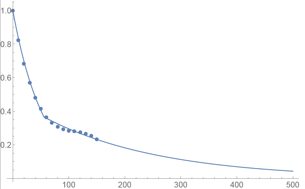
Functional Form: Amplitude vs. Calendar Days
To prevent the parametric function from becoming vanishingly small at long maturities, we apply a floor to the longer term exponential so the final implementation of this function is:
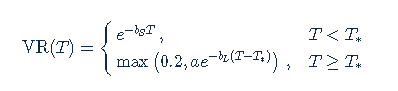
where bS=0.0180611, a=0.365678, bL=0.00482976, and T*=55.7 are obtained by fitting the main eigenvector to the parametric formula.
Inverse square root time decay
Another common approach to standardize volatility moves across maturities uses the factor 1/√T. As shown in the graph below, our house VR(T) function has a bigger volatility changes than this simplified model.
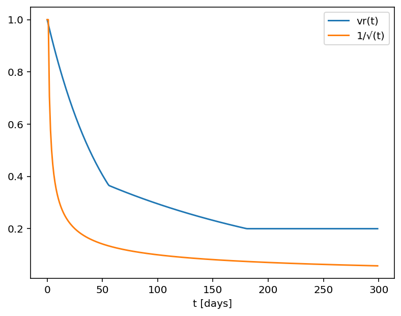
Time function comparison: Amplitude vs. Calendar Days
Adjusted Vega columns
Risk Navigator (SM) reports a computed Vega for each position; by convention, this is the p/l change per 1% increase in the volatility used for pricing. Aggregating these Vega values thus provides the portfolio p/l change for a 1% across-the-board increase in all volatilities – a parallel shift of volatility.
However, as described above a change in market volatilities might not take the form of a parallel shift. Empirically, we observe that the implied volatility of short-dated options tends to fluctuate more than that of longer-dated options. This differing sensitivity is similar to the "beta" parameter of the Capital Asset Pricing Model. We refer to this effect as term structure of volatility response.
By multiplying the Vega of an option position with an expiry-dependent quantity, we can compute a term-adjusted Vega intended to allow more accurate comparison of volatility exposures across expiries. Naturally the hoped-for increase in accuracy can only come about if the adjustment we choose turns out to accurately model the change in market implied volatility.
We offer two parametrized functions of expiry which can be used to compute this Vega adjustment to better represent the volatility sensitivity characteristics of the options as a function of time to maturity. Note that these are also referred as 'time weighted' or 'normalized' Vega.
Adjusted Vega
A column titled "Vega Adjusted" multiplies the Vega by our in-house VR(T) term structure function. This is available any option that is not a derivative of a Volatility Product ETP. Examples are SPX, IBM, VIX but not VXX.
Vega x T-1/2
A column for the same set of products as above titled "Vega x T-1/2" multiplies the Vega by the inverse square root of T (i.e. 1/√T) where T is the number of calendar days to expiry.
Aggregations
Cross over underlying aggregations are calculated in the usual fashion given the new values. Based on the selected Vega aggregation method we support None, Straight Add (SA) and Same Percentage Move (SPM). In SPM mode we summarize individual Vega values multiplied by implied volatility. All aggregation methods convert the values into the base currency of the portfolio.
Custom scenario calculation of volatility index options
Implied Volatility Indices are indexes that are computed real-time basis throughout each trading day just as a regular equity index, but they are measuring volatility and not price. Among the most important ones is CBOE's Marker Volatility Index (VIX). It measures the market's expectation of 30-day volatility implied by S&P 500 Index (SPX) option prices. The calculation estimates expected volatility by averaging the weighted prices of SPX puts and calls over a wide range of strike prices.
The pricing for volatility index options have some differences from the pricing for equity and stock index options. The underlying for such options is the expected, or forward, value of the index at expiration, rather than the current, or "spot" index value. Volatility index option prices should reflect the forward value of the volatility index (which is typically not as volatile as the spot index). Forward prices of option volatility exhibit a "term structure", meaning that the prices of options expiring on different dates may imply different, albeit related, volatility estimates.
For volatility index options like VIX the custom scenario editor of Risk Navigator offers custom adjustment of the VIX spot price and it estimates the scenario forward prices based on the current forward and VR(T) adjusted shock of the scenario adjusted index on the following way.
- Let S0 be the current spot index price, and
- S1 be the adjusted scenario index price.
- If F0 is the current real time forward price for the given option expiry, then
- F1 scenario forward price is F1 = F0 + (S1 - S0) x VR(T), where T is the number of calendar days to expiry.
Additional Information Regarding the Use of Stop Orders
U.S. equity markets occasionally experience periods of extraordinary volatility and price dislocation. Sometimes these occurrences are prolonged and at other times they are of very short duration. Stop orders may play a role in contributing to downward price pressure and market volatility and may result in executions at prices very far from the trigger price.
Investors may use stop sell orders to help protect a profit position in the event the price of a stock declines or to limit a loss. In addition, investors with a short position may use stop buy orders to help limit losses in the event of price increases. However, because stop orders, once triggered, become market orders, investors immediately face the same risks inherent with market orders – particularly during volatile market conditions when orders may be executed at prices materially above or below expected prices.
While stop orders may be a useful tool for investors to help monitor the price of their positions, stop orders are not without potential risks. If you choose to trade using stop orders, please keep the following information in mind:
· Stop prices are not guaranteed execution prices. A “stop order” becomes a “market order” when the “stop price” is reached and the resulting order is required to be executed fully and promptly at the current market price. Therefore, the price at which a stop order ultimately is executed may be very different from the investor’s “stop price.” Accordingly, while a customer may receive a prompt execution of a stop order that becomes a market order, during volatile market conditions, the execution price may be significantly different from the stop price, if the market is moving rapidly.
· Stop orders may be triggered by a short-lived, dramatic price change. During periods of volatile market conditions, the price of a stock can move significantly in a short period of time and trigger an execution of a stop order (and the stock may later resume trading at its prior price level). Investors should understand that if their stop order is triggered under these circumstances, their order may be filled at an undesirable price, and the price may subsequently stabilize during the same trading day.
· Sell stop orders may exacerbate price declines during times of extreme volatility. The activation of sell stop orders may add downward price pressure on a security. If triggered during a precipitous price decline, a sell stop order also is more likely to result in an execution well below the stop price.
· Placing a “limit price” on a stop order may help manage some of these risks. A stop order with a “limit price” (a “stop limit” order) becomes a “limit order” when the stock reaches or exceeds the “stop price.” A “limit order” is an order to buy or sell a security for an amount no worse than a specific price (i.e., the “limit price”). By using a stop limit order instead of a regular stop order, a customer will receive additional certainty with respect to the price the customer receives for the stock. However, investors also should be aware that, because a sell order cannot be filled at a price that is lower (or a buy order for a price that is higher) than the limit price selected, there is the possibility that the order will not be filled at all. Customers should consider using limit orders in cases where they prioritize achieving a desired target price more than receiving an immediate execution irrespective of price.
· The risks inherent in stop orders may be higher during illiquid market hours or around the open and close when markets may be more volatile. This may be of heightened importance for illiquid stocks, which may become even harder to sell at the then current price level and may experience added price dislocation during times of extraordinary market volatility. Customers should consider restricting the time of day during which a stop order may be triggered to prevent stop orders from activating during illiquid market hours or around the open and close when markets may be more volatile, and consider using other order types during these periods.
· In light of the risks inherent in using stop orders, customers should carefully consider using other order types that may also be consistent with their trading needs.
Non-Guaranteed Combination Orders
A combination order is a special type of order that is constructed of multiple separate positions, or ‘legs’, but executed as a single transaction. The legs of the combination may be comprised of the same position type (e.g. stock vs. stock, option vs. option or SSF vs. SSF) or different position types (e.g. stock vs. option, SSF vs. option or EFP). It’s important to note that many combination order types, while submitted via the IB trading platform as a combination, are not native to (i.e., supported by) the exchanges and therefore may not be guaranteed by IB. Accordingly, IB’s policy is to guarantee only Smart-Routed U.S. stock vs. option and option vs. option combination orders.
As combination orders which are not guaranteed are exposed to the risk of partial execution, both in terms of the quantity of legs and their balance, IB requires account holders to acknowledge the 'Non-Guaranteed' attribute at the point of order entry. There are two methods for setting this attribute:
- Method 1 - Users can select the Non-Guaranteed attribute in the Misc. section on the Order Ticket for a particular order
- Method 2 - Users can add the Non-Guaranteed column to the Order Management section of the TWS
Notes:
- Non-Guaranteed combination orders are not available for Financial Advisor allocation orders
The risk of such 'Non-Guaranteed' orders is illustrated through the example below:
Example
Assume the following quotes for a Stock vs. Stock combination order to purchase shares of Microsoft (MSFT) and sell shares of Appl (AAPL).
Current markets
MSFT - 26.30 bid, 26.31 offer
AAPL - 250.25 bid, 250.30 offer
A generic combination is created to buy 1 share AAPL and sell 1 share MSFT, the implied quote would be 223.94 bid, 224 offer.
The following order is entered:
Buy 200 AAPL, Sell 200 MSFT
Pay 224
Based on the current markets, the order would appear to be executable.
- A buy of 200 shares of AAPL are routed with a 250.30 limit. Only 100 execute.
- A sell of 200 shares of MSFT are routed with a 26.30 limit. No execution is received as the market moves to 26.29 bid.
With a Non-Guaranteed combination, the 100 shares of AAPL would be placed in the client account, even though no MSFT shares were executed. The remainder of the combination order will continue to work until executed in its entirety or until it is canceled.
WebTrader: Viewing Option Chains
How to view option chains in WebTrader
For a brief introduction to the WebTrader platform please click here
For a brief video on basic order entry using WebTrader please click here
For a brief video on how to access market depth information using WebTrader please click here
For a brief video on how to customize the WebTrader please click here
How to create option spread strategies using Stategy Builder
How to create option spread strategies using OptionTrader